Assumptions for Multiple Linear Regression
Overview
This interactive statistics module is intended to review concepts regarding assumptions in multiple linear regression.
This module is intended as to be non-technical, with the intended audience being social science undergraduates. It is also intended to supplement instruction regarding such concepts.
Learning outcomes
Coverage of each assumption has two parts:
- Assumption diagnostics
- Students will review the assumptions and some common ways of diagnosing them.
- Interactive components allow seeing how diagnostics change when assumption violations occur or are more/less severe.
- Consequences of assumption violation
- Students can change the degree of assumption violations to see the consequences on estimates of regression coefficients.
- Students should be able to say what happens to the sampling distribution (e.g., bias, standard errors) under certain assumption violations.
Assumptions for Multiple Linear Regression
NoteClick here for model equations
Recall that multiple linear regression models have the form:
\[\begin{align*} Y_{i} = \beta_0 + \beta_1 X_{1,i} + \beta_2 X_{2,i} + \cdots + \beta_J X_{J,i} + \varepsilon_i \end{align*}\]
- \(i\) is an index for a particular observation or participant
- \(J\) is the total number of predictors
- \(Y_i\) is the outcome variable
- \(\beta_0\) is the intercept
- \(\beta_1, \dots, \beta_J\) are regression coefficients
- \(X_1, \dots, X_J\) are the predictors
- \(\varepsilon_i\) is an error term
In a sample, we obtain estimates:
\[\begin{align*} Y_{i} = b_0 + b_1 X_{1,i} + b_2 X_{2,i} + \cdots + b_J X_{J,i} + e_i \end{align*}\]
- \(b_0\) and \(b_1, \dots, b_J\) are now estimates of the intercept and regression coefficients
- \(e_i\) is a residual based on the sample regression line
When conducting a multiple linear regression, we make several assumptions:
- The errors are normally distributed
- There is homogeneity of variance (or homoscedasticity): Errors have the same variance, regardless of the values of the predictor.
- There are no outliers
- The relationship between our variables is linear
- Our model is correctly specified (e.g., no missing predictors)
- There is no excess multicollinearity among the predictors
This module currently discusses the first 2 assumptions. Additional details on the other assumptions are forthcoming.
NoteAlternative formulations of the assumptions
Presentation of these assumptions sometimes varies depending on the author or source. For example,
- We do not cover assumptions necessary to interpret coefficients as causal effects.
- No outliers may not be considered an assumption separate from the normality assumption. e.g., outliers could be the result of a heavy-tailed distribution for the errors. But, typically we do want to perform some diagnostics to see whether a datapoint or two are having undue influence on the results, and thus, include an examination of outliers in this module.
Evaluating Assumption Violations
One way to understand the consequences of assumption violations is through simulation. This process is very similar to we conduct a thought experiment on how sampling distributions are constructed.
Just like the sampling distribution of the mean, regression coefficients have a sampling distribution that is based on a thought experiment:
- Collect a sample (with sample size, \(n\)) for the study, including all variables.
- For the sample, compute the estimates of the regression coefficients (\(b_0, b_1, \dots, b_J\)).
- Repeat steps 1 and 2 many, many times, each time saving the value of the regression coefficients.
The resulting estimates for each coefficient form the sampling distribution for that coefficient.
This thought experiment could also save alternative quantities at step 2, such as standard error estimates, 95% Confidence Intervals or \(p\)-values. We can then examine whether the confidence intervals actually contain the true parameter or whether the null hypothesis for certain tests is rejected or not.
In evaluating assumption violations, four quantities will be of interest in this module:
- The mean of the sampling distribution.
- The shape of the sampling distribution.
- The standard deviation or standard error of the sampling distribution.
- 95% CI coverage rates.
Bias
To examine parameter bias, we can look at the mean of the sampling distribution. If the mean of the sampling distribution is the same as the corresponding population parameter, then the estimates are unbiased. If the mean of the sampling distribution is different than the corresponding population parameter, then the estimates are biased.
For example, we can examine whether the mean of the sampling distribution is equal to \(\beta_1\) (i.e., do the estimates tend to pile up near \(\beta_1\), or around some other number?)
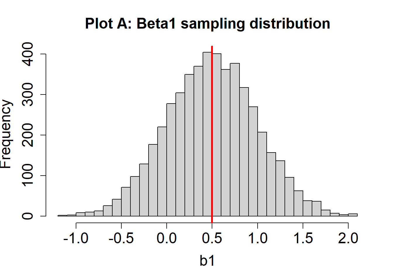
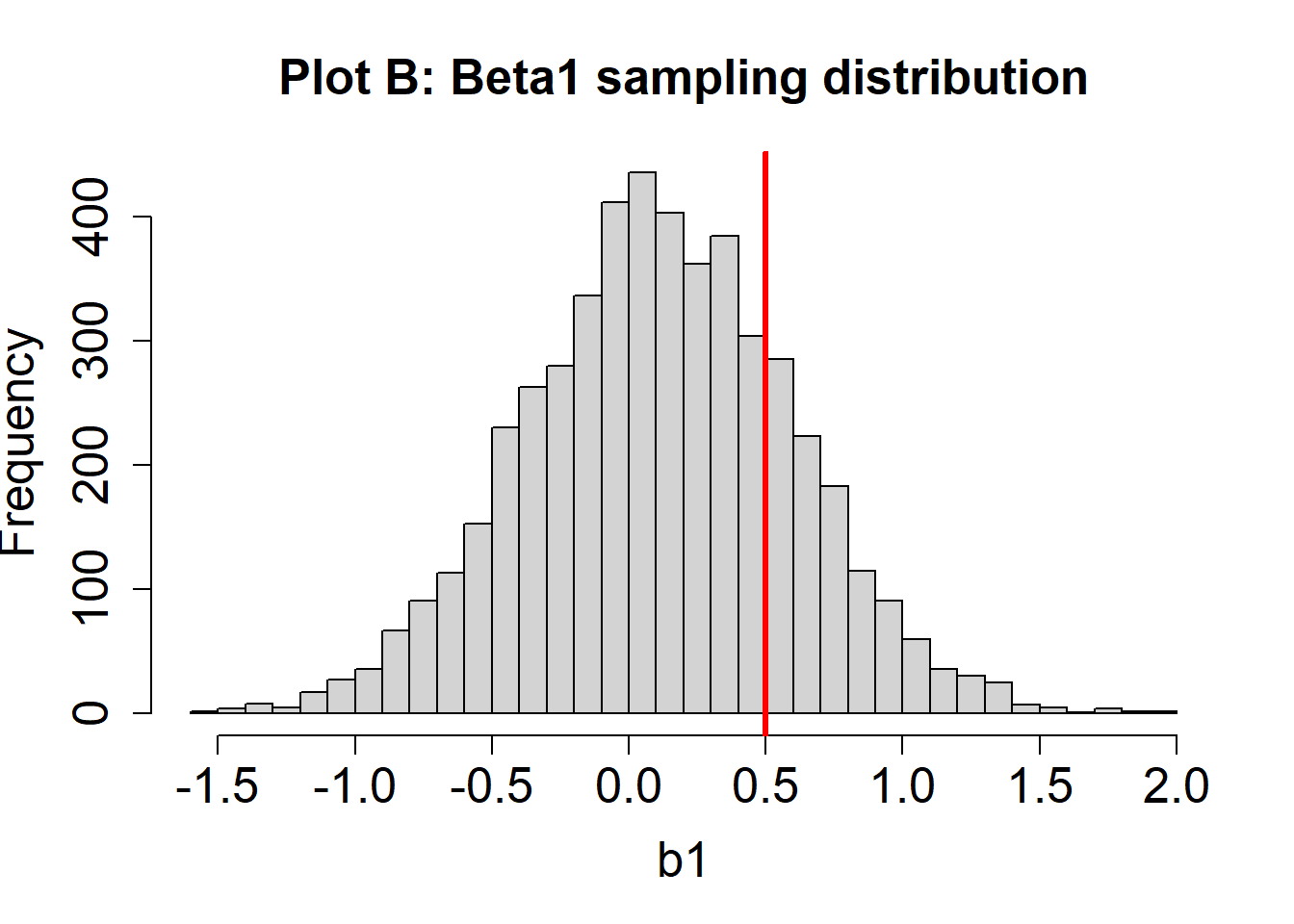
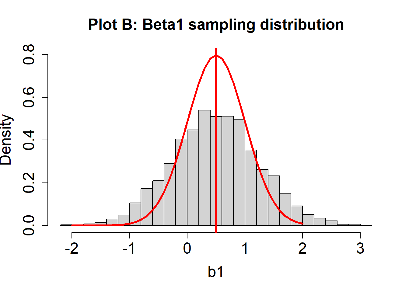
Suppose we plot a histogram of the sampling distribution for \(\beta_1\) (or many values of \(b_1\)). Suppose also that \(\beta_1 = .5\), and is indicated by a vertical red line. Two hypothetical sampling distribution plots are below.
- For the sampling distribution in Plot A, are the estimates of \(\beta_1\) unbiased? How can you know?
Click here to see answer
The estimates of \(\beta_1\) in Plot A are unbiased. We know this because the mean of the sampling distribution (about 0.5) is the same as the value of the population parameter (\(\beta_1 = 0.5\))
- For the sampling distribution in Plot B, are the estimates of \(\beta_1\) unbiased? How can you know?
Click here to see answer
The estimates of \(\beta_1\) in Plot B are biased. We know this because the mean of the sampling distribution (about 0.1) is different than the population parameter (\(\beta_1 = 0.5\)). In this case, these tend to be underestimates of the true parameter because the estimates are too small, on average.
Shape of sampling distribution
To later conduct inferences, if assumptions hold, the sampling distribution for each coefficient follows a \(t\)-distribution with the residual degrees of freedom for the model. To the naked eye, it may be difficult to tell the difference between a \(t\)-distribution and a normal distribution: both are bell-shaped, symmetric distributions. As the residual degrees of freedom increases, the \(t\)-distribution approaches a normal distribution. As such, if certain assumptions hold, the central limit theorem should kick in and sampling distributions should look normal.
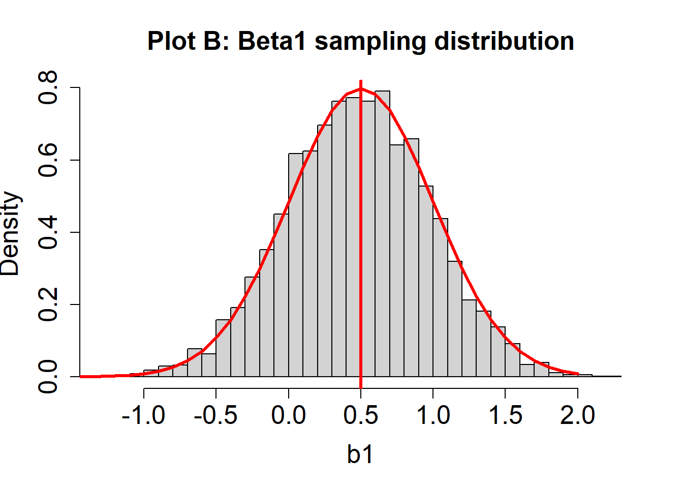
Consider again two hypothetical sampling distributions for \(\beta_1\). A red line indicating a normal distribution is overlayed.
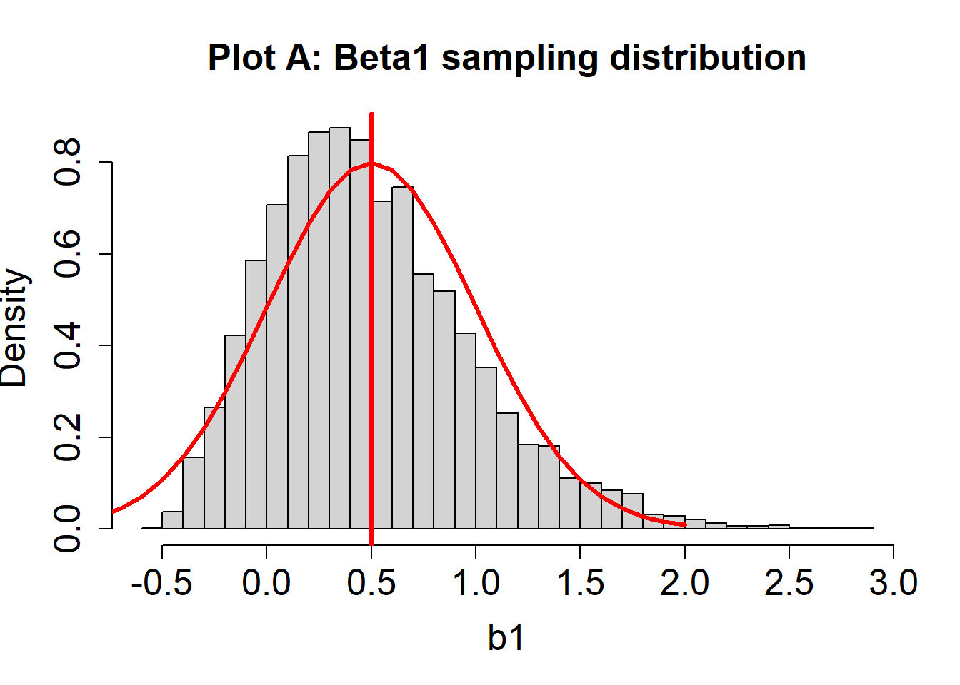
- For Plot A, does the sampling distribution for \(\beta_1\) estimates look normal?
Click here to see answer
Not exactly. You should notice a slight discrepancy between the histogram (the actual estimates of \(\beta_1\); i.e., many values of \(b_1\) from different hypothetical studies) and the red curve (signifying a normal distribution).
- For Plot B, does the sampling distribution for \(\beta_1\) estimates look normal?
Click here to see answer
In this case, the histogram and the red curve should match nicely. The sampling distribution looks approximately normal.
Standard errors
The standard error is the standard deviation of the sampling distribution. When we conduct inference for a regression coefficient based on a single sample, we need an estimate of the standard error based on just that sample. If assumptions needed to make that estimate do not hold, then the standard error estimates based on the sample may be incorrect. This may manifest in the variability for the actual sampling distribution being different than what it theoretically ought to be if the assumptions hold. For example, the actual sampling variability may be greater than the theoretical sampling variability.
Consider again two hypothetical sampling distributions for \(\beta_1\). A red line indicates the theoretical sampling distribution, if assumptions where to hold.
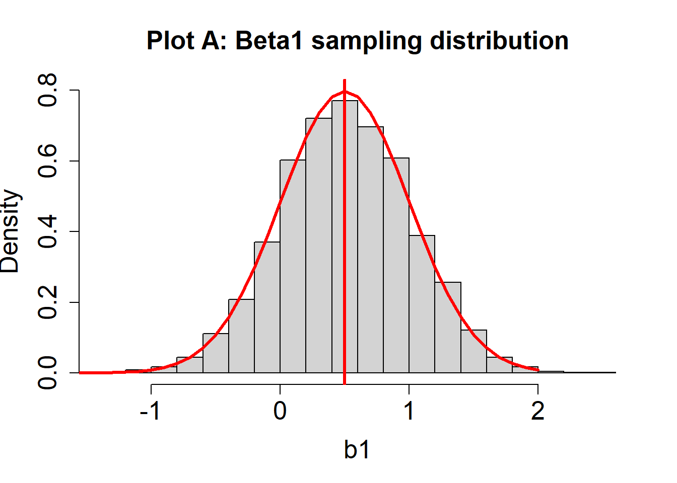
- For Plot A, does variability of the sampling distribution for \(\beta_1\) look like it matches the theoretical distribution?
Click here to see answer
Yes, the variability of the histogram should look approximately the same as that of the theoretical distribution (red line).
- For Plot B, does variability of the sampling distribution for \(\beta_1\) look like it matches the theoretical distribution?
Click here to see answer
No, the variability of the histogram should look greater than that of the theoretical distribution (red line). Note how the histogram has a lower peak and larger tails; it is more spread out.
95% CI coverage rates
Looking at histograms to evaluate bias, shape, and standard errors is sometimes difficult. Ultimately we would like to conduct inferences or form confidence intervals. An indirect way to evaluate whether all is good is to consider whether confidence intervals contain the true parameter the correct proportion of times. For example, suppose we conduct the study 1000 times, and each time we compute a 95% CI. The 95% CIs would be expected to contain the true population parameter 950/1000 of the time, or 950/1000 = .95. This proportion is the 95% CI coverage rate.
Suppose that anything below .925 is considered a low coverage rate. Low coverage rates are bad because it means that the 95% CIs are missing the true parameter many more times than we think. If the null hypothesis is true, low coverage rates also translate into high Type I error rates.
Suppose that anything above .975 is considered a high coverage rate. High coverage rates mean that the 95% CIs capture the true parameter more times than we think. Although at first glance this may not seem like a bad thing, it translates into CIs that are too wide and do not give us enough precise information about the parameter.
Later in this module, we will simply print the 95% CI coverage rate on top of the histograms of the sampling distributions. As an example, suppose 1000 simulations are conducted and here is the histogram and coverage rate for 95% CIs about \(\beta_1\):
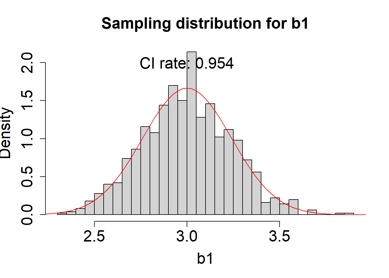
- In this example, what is the coverage rate and exactly what does it mean?
Click here to see answer
Here, the coverage rate is .954, which means that 954/1000 times the true parameter was between the lower and upper boundary of the 95% CI.
- In this example, is this a good coverage rate?
Click here to see answer
Yes, .954 is very close to .95, the desired coverage rate.
- If a coverage were to be .87, would this be good?
Click here to see answer
No, .87 is too low of a coverage rate (If we follow the rule of thumb presented earlier, it is below .925). It would mean that only 870/1000 times the CI contained the true population parameter.
Looking ahead
For the remaining modules, you will examine diagnostics for regression analysis assumptions. In addition, you will look at whether assumption violations have consequences for the estimates of the regression coefficients or their inferences by looking at the sampling distributions or the CI coverage rates.
Normally Distributed Errors
The first assumption is that the errors in the population follow a normal distribution, with a mean of zero.
\[ \varepsilon_i \sim N(0,\sigma^2)\] That is, “the errors (\(\varepsilon_i\)) follow a normal distribution with a mean of zero and some constant variance”.
Q-Q Plots
Since we do not have the errors in the population, the best we can do is look at residuals in our sample.
The most commonly recommended way to assess this assumption is the Quantile-Quantile Plot or Q-Q Plot.
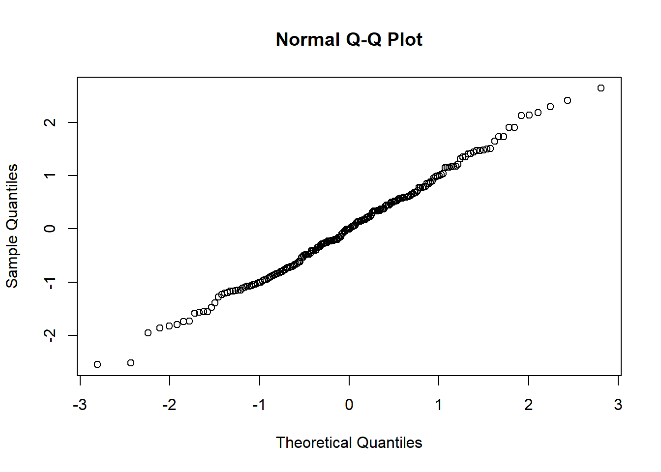
The y-axis of a normal Q-Q plot from multiple linear regression represents the (quantiles of) standardized residuals from our model.
The x-axis of a normal Q-Q plot represents theoretical quantiles, or what the standardized residuals would look like if they perfectly followed a normal distribution.
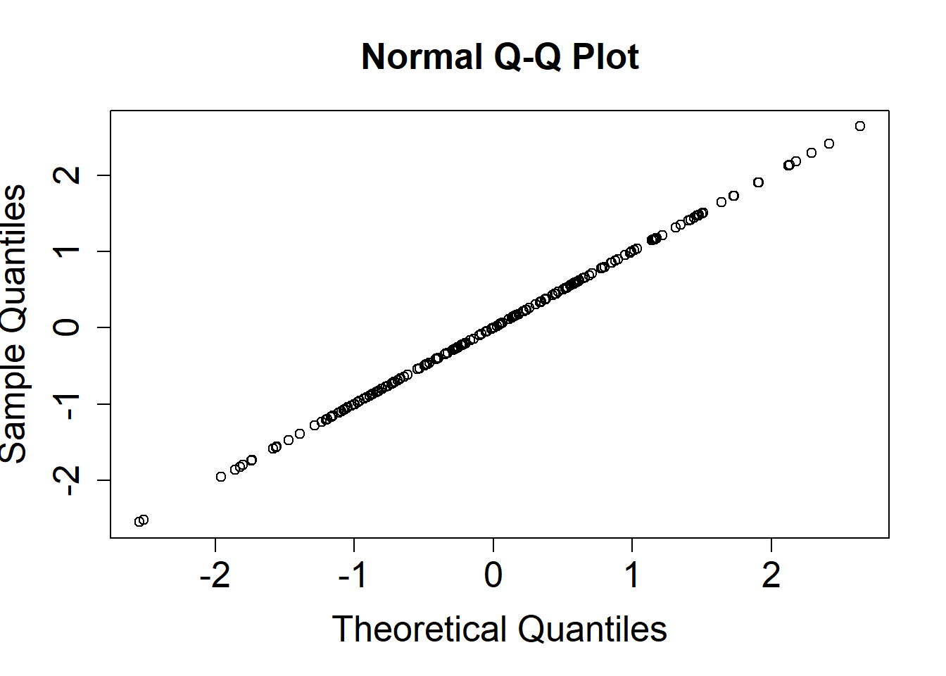
If our residuals perfectly follow a normal distribution, our Q-Q plot will be a straight line.
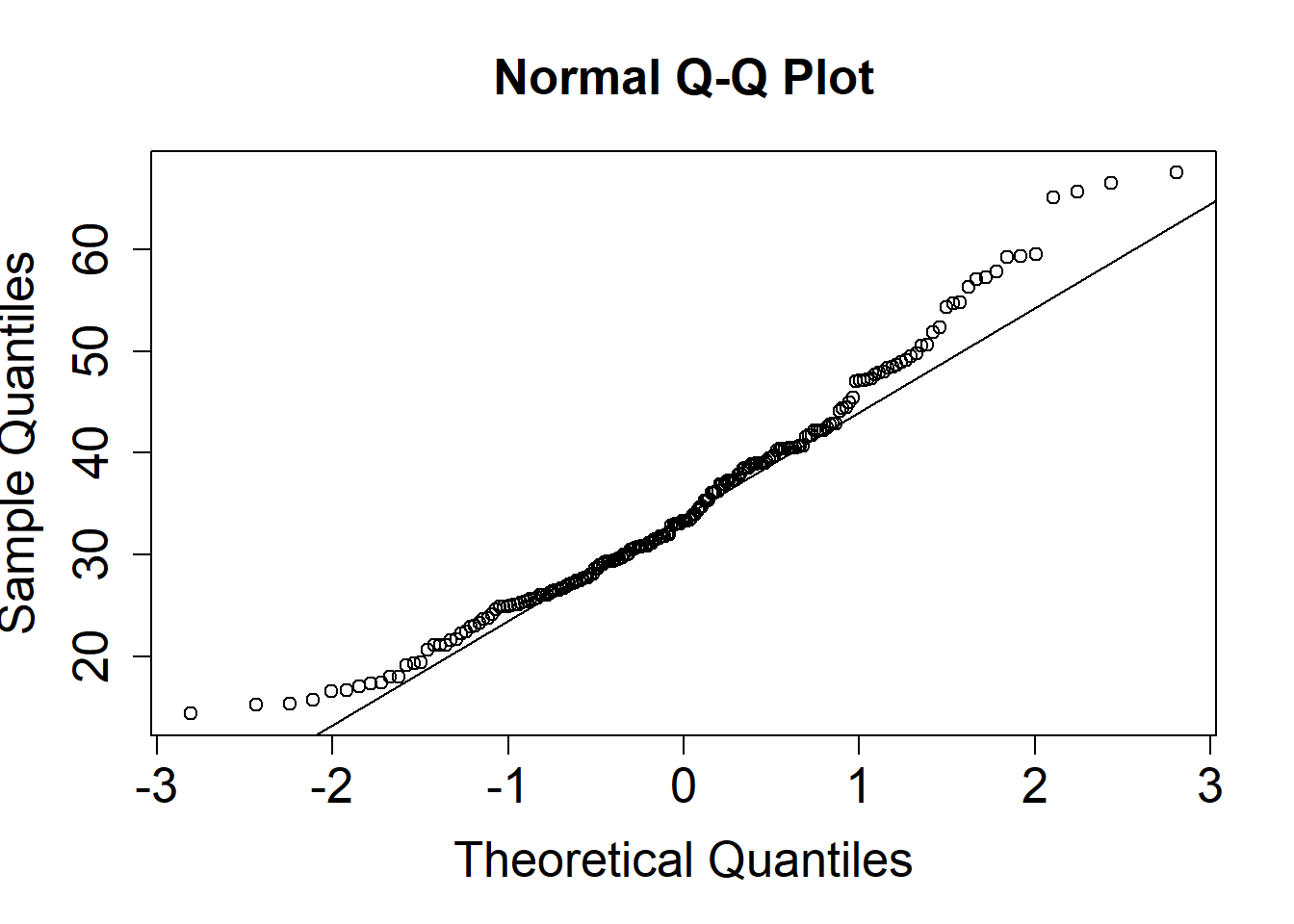
The more our residuals are non-normal, the more the datapoints will deviate from a straight line.
Histograms of residuals
Another way of assessing normality is to visualize the standardized residuals in a histogram
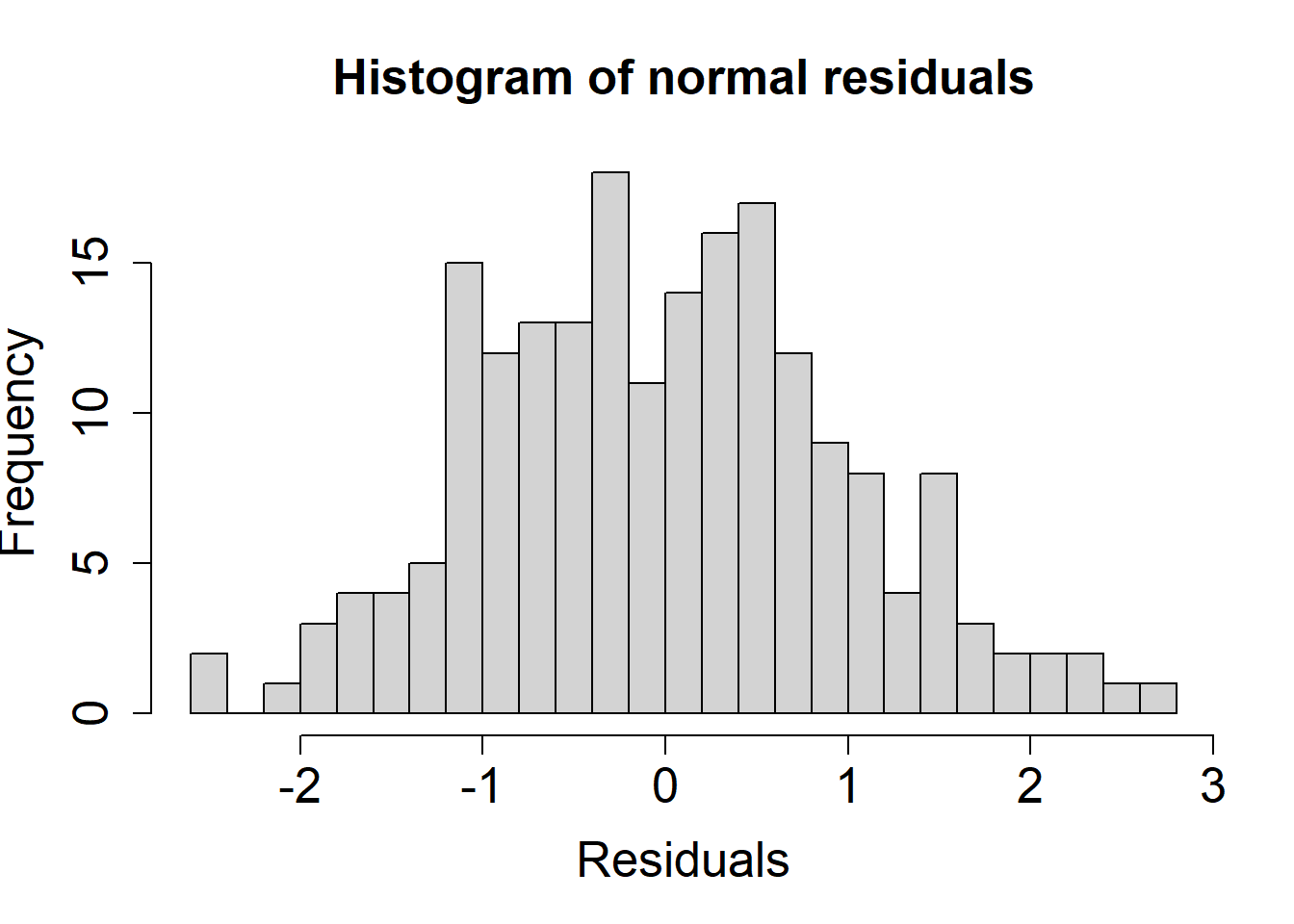
Here, we can see the residuals follow a normal distribution.
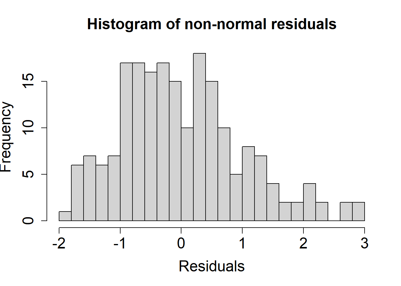
Here, we can see the residuals do not follow a normal distribution.
Amount of nonnormality
Interpreting Q-Q plots is necessarily an art; try adjusting the degree of non-normality to see how the plots of the residuals change.
#| '!! shinylive warning !!': |
#|   shinylive does not work in self-contained HTML documents.
#|   Please set `embed-resources: false` in your metadata.
#| standalone: true
#| viewerHeight: 500

library(tibble) # CFF: this one also apparently required for shinylive to work sometimes
library(dplyr)
library(shiny)
library(munsell) # was included due to bug in getting ggplot2 to work with shinylive; still required for some reason
library(ggplot2)

#library(covsim) # initially used for nonnormality, but not available
# To see what packages are available: https://repo.r-wasm.org/

#------------------------------------------------------------------
## Functions modified from semTools
library(mnormt)
mvrnonnorm <- function (n, mu, Sigma, skewness = NULL, kurtosis = NULL, empirical = FALSE)
{
  p <- length(mu)
  if (!all(dim(Sigma) == c(p, p)))
    stop("incompatible arguments")
  varnames <- names(mu)
  if (is.null(varnames))
    varnames <- rownames(Sigma)
  if (is.null(varnames))
    varnames <- colnames(Sigma)
  eS <- eigen(Sigma, symmetric = TRUE)
  ev <- eS$values
  if (!all(ev >= -1e-06 * abs(ev[1L])))
    stop("'Sigma' is not positive definite")
  if (is.null(skewness) && is.null(kurtosis)) {
    X <- mnormt::rmnorm(n = n, mean = mu, varcov = Sigma)
  }
  else {
    if (is.null(skewness))
      skewness <- rep(0, p)
    if (is.null(kurtosis))
      kurtosis <- rep(0, p)
    Z <- ValeMaurelli1983copied(n = n, COR = cov2cor(Sigma),
                                skewness = skewness, kurtosis = kurtosis)
    TMP <- scale(Z, center = FALSE, scale = 1/sqrt(diag(Sigma)))[,
                                                                 , drop = FALSE]
    X <- sweep(TMP, MARGIN = 2, STATS = mu, FUN = "+")
  }
  colnames(X) <- varnames
  X
}

ValeMaurelli1983copied <- function (n = 100L, COR, skewness, kurtosis, debug = FALSE)
{
  fleishman1978_abcd <- function(skewness, kurtosis) {
    system.function <- function(x, skewness, kurtosis) {
      b. = x[1L]
      c. = x[2L]
      d. = x[3L]
      eq1 <- b.^2 + 6 * b. * d. + 2 * c.^2 + 15 * d.^2 -
        1
      eq2 <- 2 * c. * (b.^2 + 24 * b. * d. + 105 * d.^2 +
                         2) - skewness
      eq3 <- 24 * (b. * d. + c.^2 * (1 + b.^2 + 28 * b. *
                                       d.) + d.^2 * (12 + 48 * b. * d. + 141 * c.^2 +
                                                       225 * d.^2)) - kurtosis
      eq <- c(eq1, eq2, eq3)
      sum(eq^2)
    }
    out <- nlminb(start = c(1, 0, 0), objective = system.function,
                  scale = 10, control = list(trace = 0), skewness = skewness,
                  kurtosis = kurtosis)
    if (out$convergence != 0)
      warning("no convergence")
    b. <- out$par[1L]
    c. <- out$par[2L]
    d. <- out$par[3L]
    a. <- -c.
    c(a., b., c., d.)
  }
  getICOV <- function(b1, c1, d1, b2, c2, d2, R) {
    objectiveFunction <- function(x, b1, c1, d1, b2, c2,
                                  d2, R) {
      rho = x[1L]
      eq <- rho * (b1 * b2 + 3 * b1 * d2 + 3 * d1 * b2 +
                     9 * d1 * d2) + rho^2 * (2 * c1 * c2) + rho^3 *
        (6 * d1 * d2) - R
      eq^2
    }
    out <- nlminb(start = R, objective = objectiveFunction,
                  scale = 10, control = list(trace = 0), b1 = b1,
                  c1 = c1, d1 = d1, b2 = b2, c2 = c2, d2 = d2, R = R)
    if (out$convergence != 0)
      warning("no convergence")
    rho <- out$par[1L]
    rho
  }
  nvar <- ncol(COR)
  if (is.null(skewness)) {
    SK <- rep(0, nvar)
  }
  else if (length(skewness) == nvar) {
    SK <- skewness
  }
  else if (length(skewness) == 1L) {
    SK <- rep(skewness, nvar)
  }
  else {
    stop("skewness has wrong length")
  }
  if (is.null(kurtosis)) {
    KU <- rep(0, nvar)
  }
  else if (length(kurtosis) == nvar) {
    KU <- kurtosis
  }
  else if (length(kurtosis) == 1L) {
    KU <- rep(kurtosis, nvar)
  }
  else {
    stop("kurtosis has wrong length")
  }
  FTable <- matrix(0, nvar, 4L)
  for (i in 1:nvar) {
    FTable[i, ] <- fleishman1978_abcd(skewness = SK[i],
                                      kurtosis = KU[i])
  }
  # For this demo, didn't care whether variance was maintained, and didn't check

  X <- Z <- mnormt::rmnorm(n = n, mean = rep(0, nvar), varcov = COR)
  X <- FTable[1, 1L] + FTable[1, 2L] * Z + FTable[i,3L] * Z^2 + FTable[i, 4L] * Z^3
  X
}
# End of functions modified from semTools
#------------------------------------------------------------------

ui <- fluidPage(
    fluidRow(
        column(width = 6,
            plotOutput("qqPlot")),
        column(width = 6,
            plotOutput(outputId = "histPlot"))
    ),
    fluidRow(
      column(width = 12,
             sliderInput("skew", "Skewness", min=-1, max=1, value=0, step=.1))
    )
)

server <- function(input, output){
  datskew <- reactive({
    set.seed(2025)
    skew <- input$skew
    #tmp <- rnorm(1000)
    tmp <- mvrnonnorm(1000, as.vector(0), diag(1), skewness=skew, kurtosis = 0)
    #tmp <- covsim::rIG(1000, diag(1), skew, excesskurtosis = 0)[[1]]
    return(tmp)
  })

  output$qqPlot <-  renderPlot({
    qqnorm(datskew(),
        cex.lab = 1.6, cex.axis = 1.6, cex.main = 1.6)
    qqline(datskew())
  })

  output$histPlot <-  renderPlot({
    hist(datskew(), main = "Histogram",
        cex.lab = 1.6, cex.axis = 1.6, cex.main = 1.6,
        xlab = "Residuals",
        breaks = 25)
  })

}

shinyApp(ui, server)
#| '!! shinylive warning !!': |
#|   shinylive does not work in self-contained HTML documents.
#|   Please set `embed-resources: false` in your metadata.
#| standalone: true
#| viewerHeight: 500

library(tibble) # CFF: this one also apparently required for shinylive to work sometimes
library(dplyr)
library(shiny)
library(munsell) # was included due to bug in getting ggplot2 to work with shinylive; still required for some reason
library(ggplot2)

#library(covsim) # initially used for nonnormality, but not available
# To see what packages are available: https://repo.r-wasm.org/

#------------------------------------------------------------------
## Functions modified from semTools
library(mnormt)
mvrnonnorm <- function (n, mu, Sigma, skewness = NULL, kurtosis = NULL, empirical = FALSE)
{
  p <- length(mu)
  if (!all(dim(Sigma) == c(p, p)))
    stop("incompatible arguments")
  varnames <- names(mu)
  if (is.null(varnames))
    varnames <- rownames(Sigma)
  if (is.null(varnames))
    varnames <- colnames(Sigma)
  eS <- eigen(Sigma, symmetric = TRUE)
  ev <- eS$values
  if (!all(ev >= -1e-06 * abs(ev[1L])))
    stop("'Sigma' is not positive definite")
  if (is.null(skewness) && is.null(kurtosis)) {
    X <- mnormt::rmnorm(n = n, mean = mu, varcov = Sigma)
  }
  else {
    if (is.null(skewness))
      skewness <- rep(0, p)
    if (is.null(kurtosis))
      kurtosis <- rep(0, p)
    Z <- ValeMaurelli1983copied(n = n, COR = cov2cor(Sigma),
                                skewness = skewness, kurtosis = kurtosis)
    TMP <- scale(Z, center = FALSE, scale = 1/sqrt(diag(Sigma)))[,
                                                                 , drop = FALSE]
    X <- sweep(TMP, MARGIN = 2, STATS = mu, FUN = "+")
  }
  colnames(X) <- varnames
  X
}

ValeMaurelli1983copied <- function (n = 100L, COR, skewness, kurtosis, debug = FALSE)
{
  fleishman1978_abcd <- function(skewness, kurtosis) {
    system.function <- function(x, skewness, kurtosis) {
      b. = x[1L]
      c. = x[2L]
      d. = x[3L]
      eq1 <- b.^2 + 6 * b. * d. + 2 * c.^2 + 15 * d.^2 -
        1
      eq2 <- 2 * c. * (b.^2 + 24 * b. * d. + 105 * d.^2 +
                         2) - skewness
      eq3 <- 24 * (b. * d. + c.^2 * (1 + b.^2 + 28 * b. *
                                       d.) + d.^2 * (12 + 48 * b. * d. + 141 * c.^2 +
                                                       225 * d.^2)) - kurtosis
      eq <- c(eq1, eq2, eq3)
      sum(eq^2)
    }
    out <- nlminb(start = c(1, 0, 0), objective = system.function,
                  scale = 10, control = list(trace = 0), skewness = skewness,
                  kurtosis = kurtosis)
    if (out$convergence != 0)
      warning("no convergence")
    b. <- out$par[1L]
    c. <- out$par[2L]
    d. <- out$par[3L]
    a. <- -c.
    c(a., b., c., d.)
  }
  getICOV <- function(b1, c1, d1, b2, c2, d2, R) {
    objectiveFunction <- function(x, b1, c1, d1, b2, c2,
                                  d2, R) {
      rho = x[1L]
      eq <- rho * (b1 * b2 + 3 * b1 * d2 + 3 * d1 * b2 +
                     9 * d1 * d2) + rho^2 * (2 * c1 * c2) + rho^3 *
        (6 * d1 * d2) - R
      eq^2
    }
    out <- nlminb(start = R, objective = objectiveFunction,
                  scale = 10, control = list(trace = 0), b1 = b1,
                  c1 = c1, d1 = d1, b2 = b2, c2 = c2, d2 = d2, R = R)
    if (out$convergence != 0)
      warning("no convergence")
    rho <- out$par[1L]
    rho
  }
  nvar <- ncol(COR)
  if (is.null(skewness)) {
    SK <- rep(0, nvar)
  }
  else if (length(skewness) == nvar) {
    SK <- skewness
  }
  else if (length(skewness) == 1L) {
    SK <- rep(skewness, nvar)
  }
  else {
    stop("skewness has wrong length")
  }
  if (is.null(kurtosis)) {
    KU <- rep(0, nvar)
  }
  else if (length(kurtosis) == nvar) {
    KU <- kurtosis
  }
  else if (length(kurtosis) == 1L) {
    KU <- rep(kurtosis, nvar)
  }
  else {
    stop("kurtosis has wrong length")
  }
  FTable <- matrix(0, nvar, 4L)
  for (i in 1:nvar) {
    FTable[i, ] <- fleishman1978_abcd(skewness = SK[i],
                                      kurtosis = KU[i])
  }
  # For this demo, didn't care whether variance was maintained, and didn't check

  X <- Z <- mnormt::rmnorm(n = n, mean = rep(0, nvar), varcov = COR)
  X <- FTable[1, 1L] + FTable[1, 2L] * Z + FTable[i,3L] * Z^2 + FTable[i, 4L] * Z^3
  X
}
# End of functions modified from semTools
#------------------------------------------------------------------

ui <- fluidPage(
  fluidRow(
    column(width = 6,
           plotOutput(outputId = "qqPlot2")),
    column(width = 6,
           plotOutput(outputId = "histPlot2"))
  ),
  sliderInput("kurt", "(Excess) Kurtosis", min=-1, max=3, value=0, step=.5)
)

server <- function(input, output){


  datskew2 <- reactive({
    set.seed(2025)
    kurtosis <- input$kurt
    tmp <- mvrnonnorm(1000, 0, diag(1), skewness=0, kurtosis = kurtosis)
    #tmp <- rIG(1000, diag(1), skew=0, excesskurtosis = kurtosis)[[1]]
    return(tmp)
  })


  output$qqPlot2 <-  renderPlot({
   qqnorm(datskew2(),
     cex.lab = 1.6, cex.axis = 1.6, cex.main = 1.6)
   qqline(datskew2())
  })

  output$histPlot2 <-  renderPlot({
   hist(datskew2(), main = "Histogram",
     cex.lab = 1.6, cex.axis = 1.6, cex.main = 1.6,
     xlab = "Residuals",
     breaks = 25, xlim=c(-4,4), ylim = c(0, 225))
  })

}

shinyApp(ui, server)
Consequences of non-normal errors
Suppose we have a simple model:
\[\begin{align*} Y_{i} = \beta_0 + \beta_1 X_{1,i} + \varepsilon_i \end{align*}\]
Assume:
- \(\beta_0 = 2\)
- \(\beta_1 = 3\)
We collect \(n=15\) participants and estimate a regression model. We repeat this many times to create a sampling distribution, including both \(b_0\) and \(b_1\) values.
Try adjusting the type of non-normality for the errors to see how it affects the sampling distribution. (Be patient, this part uses simulations).
#| '!! shinylive warning !!': |
#|   shinylive does not work in self-contained HTML documents.
#|   Please set `embed-resources: false` in your metadata.
#| standalone: true
#| viewerHeight: 500

library(tibble) # CFF: this one also apparently required for shinylive to work sometimes
library(dplyr)
library(shiny)
library(munsell) # was included due to bug in getting ggplot2 to work with shinylive; still required for some reason
library(ggplot2)

ui <- fluidPage(
  plotOutput(outputId = "samplingDistNormalityPlot"),
  textOutput(outputId = "nonNormality"),
  radioButtons("nntype1", "Type of Non-normality",
             choices = c("Normal","Chi-square", "Exponential"))
)

server <- function(input, output){

  nsamples <- 2500 #10000
  sample_size <- 15
  b0 <- 2
  b1 <- 3

  # settings that control error variance
  # care must be taken so that these match ok
  sigma2 <- 6
  df <- sigma2/2
  expmean <- sqrt(sigma2)

  #df <- 3.125
  #expmean <- 2.5
  #sigma2 <- 2.5^2

  #TODO: consider just generate all samples when loading

  output$samplingDistNormalityPlot <- renderPlot({

    est <- se.est <- ci.est0 <- ci.est1 <- pvals <- matrix(0,nrow=nsamples,ncol=2)
    x <- runif(sample_size,1,sample_size) # fixed predictors
    X <- cbind(rep(1,sample_size), x)
    nntype <- input$nntype1

    for (i in 1:nsamples) {
      if(nntype == "Normal"){
        y <- b0 + b1*x + rnorm(sample_size, 0, sqrt(sigma2))
        mod <- lm(y ~ x)
      } else if (nntype == "Chi-square") {
        y <- b0 + b1*x + (rchisq(sample_size, df = df) - df)
        mod <- lm(y ~ x)
      } else if (nntype == "Exponential"){
        meanval <- expmean
        y <- b0 + b1*x + rexp(sample_size, rate = 1/meanval) - meanval
        mod <- lm(y ~ x)
      }
      est[i,] <- coef(mod)
      se.est[i,] <- sqrt(diag(vcov(mod)))
      ci.est0[i,] <- confint(mod)[1,]
      ci.est1[i,] <- confint(mod)[2,]
      pvals[i,] <- summary(mod)$coefficients[,4]
    }

    # Theoretical SEs
    info <- solve((t(X)%*%X))
    ses <- sqrt(diag(info*sigma2))
    xgrid0 <- seq(b0-3, b0+3, .1)
    xgrid1 <- seq(b1-1, b1+1, .025)

    par(mfrow = c(1, 2))
    hist(est[,1], breaks=30, probability = TRUE,
         main = "Sampling distribution for b0",
         xlab = "b0",
         cex.lab = 1.7, cex.axis = 1.7, cex.main = 1.7,
         ylim=c(0,.33))
    abline(v = b0, col="red", lwd=3)
    lines(xgrid0, dnorm(xgrid0, b0, ses[1]), col="red")
    CIrate0 <- sum(ci.est0[,1] < b0 & ci.est0[,2] > b0)/nsamples
    text(.5, .27, label=paste0("CI rate: ", round(CIrate0,3) ),
         cex=1.7)


    hist(est[,2], breaks=30, probability = TRUE,
         main = "Sampling distribution for b1",
         xlab = "b1",
         cex.lab = 1.7, cex.axis = 1.7, cex.main = 1.7,
         ylim = c(0, 3.1))
    abline(v = b1, col="red", lwd=3)
    lines(xgrid1, dnorm(xgrid1, b1, ses[2]), col="red")
    CIrate1 <- sum(ci.est1[,1] < b1 & ci.est1[,2] > b1)/nsamples
    text(2.7, 2.75, label=paste0("CI rate: ", round(CIrate1,3) ),
         cex=1.7)

  })
}

shinyApp(ui, server)- When the errors are normal, do you notice any problems?
Click here to see answer
Estimates for both coefficients should be:
- Unbiased
- Normal
- Have appropriate variability
- Have 95% CI coverage rates that are not too far from .95
- When the errors are chi-square distributed, do you notice any problems?
Click here to see answer
Estimates for \(\beta_1\) (i.e., many estimates, \(b_1\)) should clearly be:
- Unbiased
- Normal
- Have appropriate variability
- Have 95% CI coverage rates that are not too far from .95
Sometimes the sampling distribution for \(b_0\) (i.e., estimates of \(\beta_0\)) can sometimes look a tiny bit non-normal. Because of the slight non-normality, it is difficult to tell whether the estimates are unbiased or whether the standard error (variability) looks correct. But, the difference is so slight that 95% CI coverage rates are usually good; sometimes these are only slightly below .95 but not lower than .925.
- When the errors come from an exponential distribution, do you notice any problems?
Click here to see answer
Estimates for \(\beta_1\) (i.e., many estimates, \(b_1\)) should clearly be:
- Unbiased
- Normal
- Have appropriate variability
- Have 95% CI coverage rates that are not too far from .95
Sometimes the sampling distribution for \(b_0\) (i.e., estimates of \(\beta_0\)) can sometimes look a tiny bit non-normal. Because of the slight non-normality, it is difficult to tell whether the estimates are unbiased or whether the standard error (variability) looks correct. But, the difference is so slight that 95% CI coverage rates are usually good; sometimes these are only slightly below .95 but not lower than .925.
- Based on just the above results, would you conclude that violations of the normality assumption are a huge problem for multiple linear regression?
Click here to see answer
Based on just these results, it does not appear that normality is a big problem. We might say that multiple linear regression is somewhat “robust” to violations of the normality assumption. The model should still result in unbiased estimates. Inferences may sometimes be more incorrect, but this appears to happen in rather extreme cases in small samples. That said, there are cases or very extreme examples where one may choose a different modeling approach to accommodate non-normality.
Homoscedasticity
The homogeneity of variance assumption is often called homoscedasticity in the context of multiple linear regression. The assumption means that the spread of the errors is the same regardless of the values of the predictor(s). This assumption is implicit in the notation, \(\varepsilon_i \sim N(0,\sigma^2)\). The variance of the errors is just \(\sigma^2\), even if \(X_1 = 0\) or \(X_1 = 5\). If this assumption is violated, it is often said that heteroscedasticity is present.
Residual plots
A common way to diagnose issues regarding homoscedasticity is again to work with the residuals in our sample. When \(J>1\), or the number of predictors is greater than 1, it can be difficult to visualize the residuals at different values of the predictors. For this reason, it is more common to use a lower-dimensional proxy for the values of the predictors. In particular, we usually visualize the residuals at different values of \(\hat{Y}_i\). Different values for \(\hat{Y}_i\) are the predicted values or fitted values of the outcome variable.
Here, we visualize the variance of residuals with a Residuals vs. Fitted Values plot. The goal is to tell whether the residuals have similar spread, regardless of the fitted values. In other words, examine the vertical spread of the points at any given value of the x-axis. Below are two hypothetical residual plots.
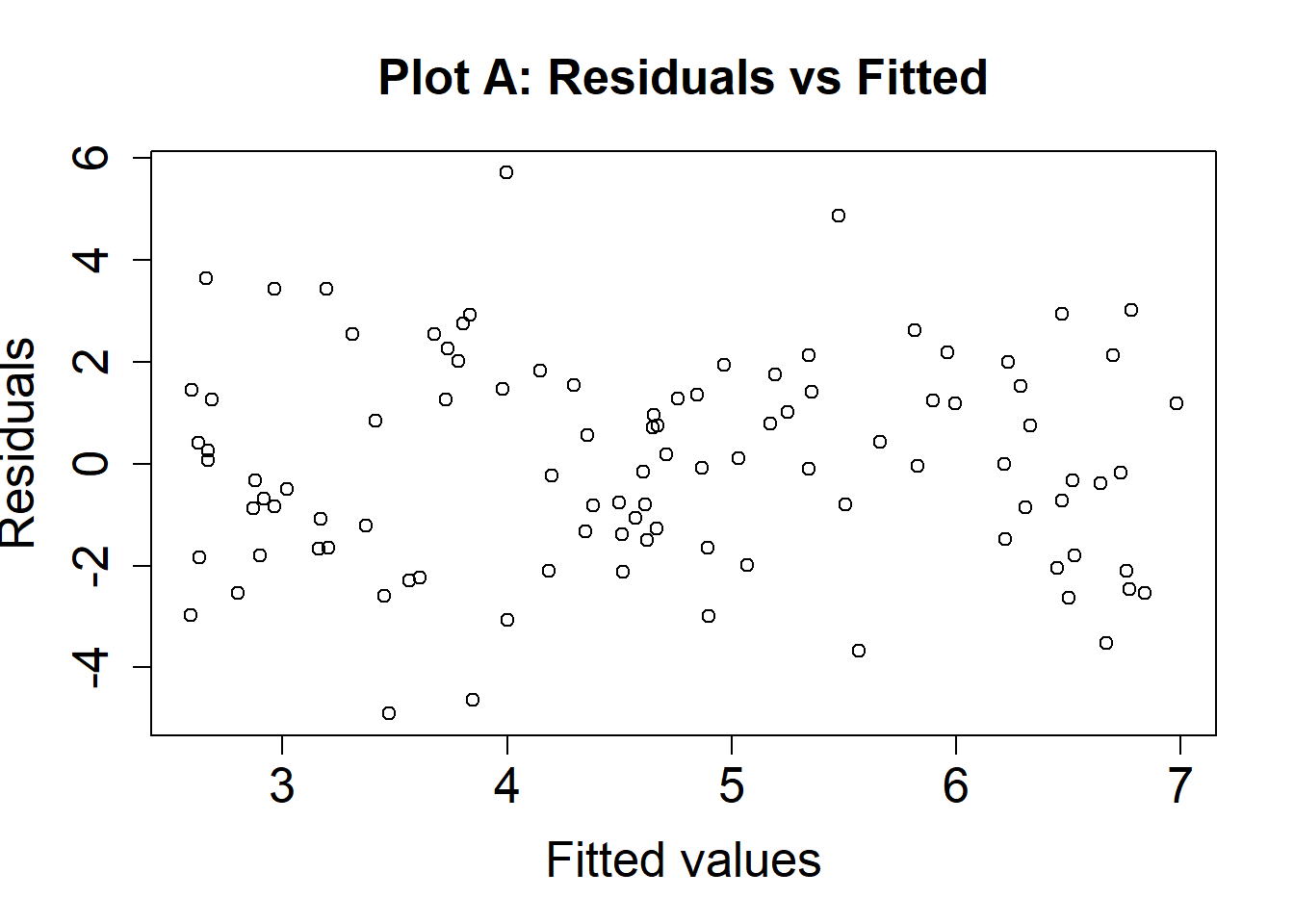
Here is an example where the assumption is met (the variability of our residuals is approximately the same across all values of the fitted values, \(\hat{Y}\)).
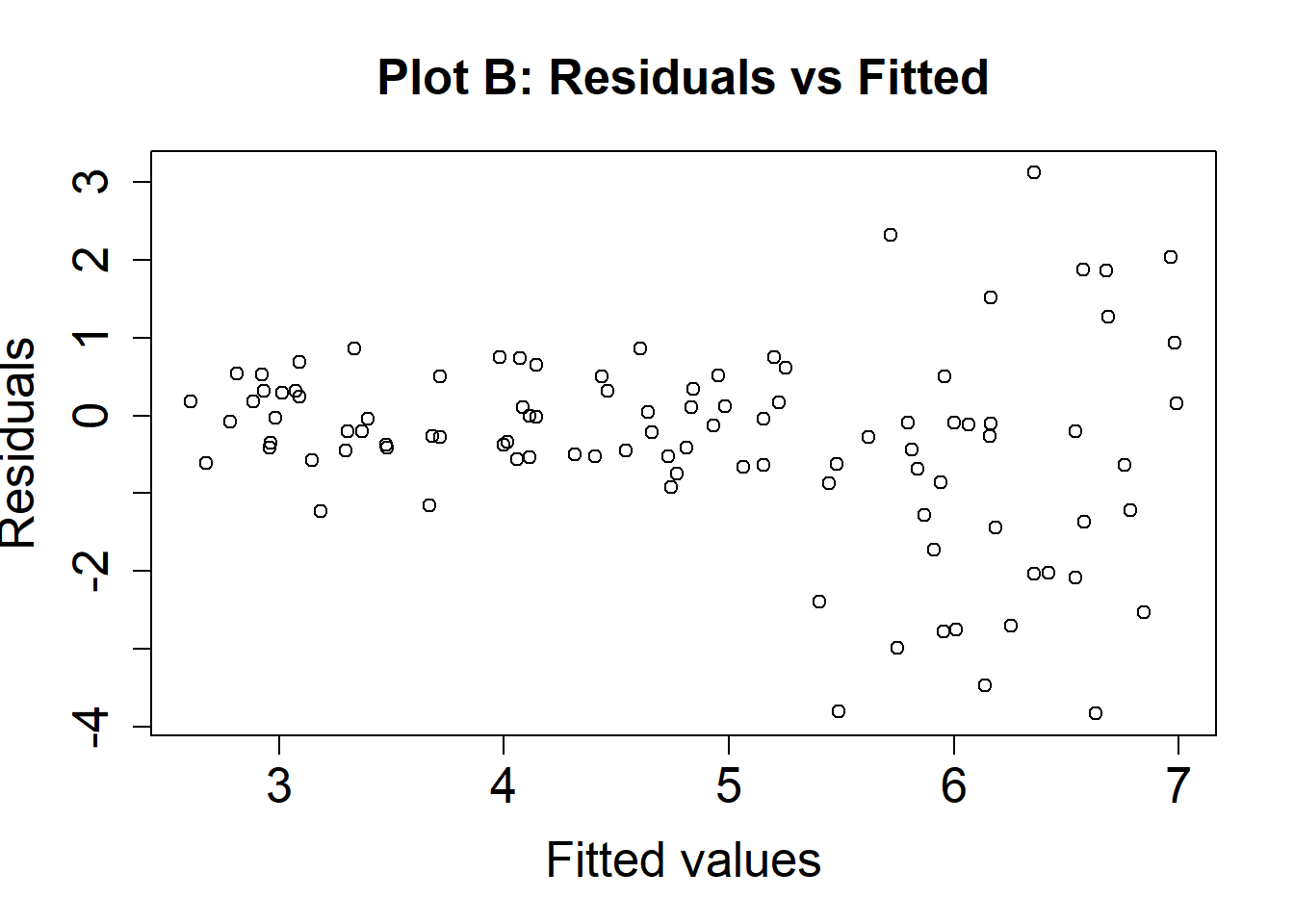
Here is an example where homoscedasticity is violated (there is more variability for higher levels of \(\hat{Y}\) compared to lower levels of the fitted values, \(\hat{Y}\)).
NoteResiduals or standardized residuals?
Some software will plot: 1) the residuals versus fitted values; or 2) the standardized residuals versus fitted values; or 3) both types of plots. Either is ok for visualizing whether the homoscedasticity assumption holds. Sometimes some patterns are easier to see in one plot versus the other.
Pattern and degree of heteroscedasticity
Interpreting residual plots is also challenging. Variability may be greater on either side of the residual plot and at low levels may be difficult to detect. Try adjusting the degree of heteroscedasticity to see how the plots of the residuals change.
#| '!! shinylive warning !!': |
#|   shinylive does not work in self-contained HTML documents.
#|   Please set `embed-resources: false` in your metadata.
#| standalone: true
#| viewerHeight: 500

library(tibble) # CFF: this one also apparently required for shinylive to work sometimes
library(dplyr)
library(shiny)
library(munsell) # was included due to bug in getting ggplot2 to work with shinylive; still required for some reason
library(ggplot2)

ui <- fluidPage(
  fluidRow(
    column(width = 6,
      plotOutput(outputId = "hetPlot1"))
  ),
  sliderInput("het", "Heteroscedasticity", min=0, max=1, value=0, step=.1)
)

server <- function(input, output){
  N <- 100
  X <- runif(N, 0, 1) # fixed X
  b0 <- 2
  b1 <- 3

  dathet1 <- reactive({
    Yhat <- b0 + b1*X
    resid <- rnorm(N, 0, sd=exp(input$het*Yhat)) # generate heteroscedastic resids
    Y <- Yhat + resid
    return(list(X = X, Y = Y))
  })

  output$hetPlot1 <-  renderPlot({
   dat <- dathet1()
   reg <- lm(dat$Y ~ dat$X)
   plot(reg, 1)

  })

}

shinyApp(ui, server)
Variability also need not be just on the right or left side of the residual plot.
#| '!! shinylive warning !!': |
#|   shinylive does not work in self-contained HTML documents.
#|   Please set `embed-resources: false` in your metadata.
#| standalone: true
#| viewerHeight: 600

library(tibble) # CFF: this one also apparently required for shinylive to work sometimes
library(dplyr)
library(shiny)
library(munsell) # was included due to bug in getting ggplot2 to work with shinylive; still required for some reason
library(ggplot2)

ui <- fluidPage(
  fluidRow(
    column(width = 6,
      plotOutput(outputId = "hetPlot2"))
  ),
  radioButtons("hetloc", "Location", choices=c("Middle Variance Higher","Middle Variance Lower")),
  sliderInput("het2", "Heteroscedasticity", min=0, max=2, value=0, step=.5)
)

server <- function(input, output){

  N <- 100
  X <- runif(N, -1, 1) # fixed X
  b0 <- 2
  b1 <- 3

  dathet2 <- reactive({
    Yhat <- b0 + b1*X
    if(input$hetloc == "Middle Variance Higher"){
      resid <- rnorm(N, 0, sd=exp(input$het2*(1-abs(X))))
    } else {
      resid <- rnorm(N, 0, sd=exp(input$het2*abs(X)))
    }
    Y <- Yhat + resid
    return(list(X = X, Y = Y))
  })

  output$hetPlot2 <-  renderPlot({
   dat <- dathet2()
   reg <- lm(dat$Y ~ dat$X)
   plot(reg, 1)

  })
}

shinyApp(ui, server)
Consequences of heteroscedasticity
Suppose we have the model:
\[\begin{align*} Y_{i} = \beta_0 + \beta_1 X_{1,i} + \beta_2 X_{2,i} + \varepsilon_i \end{align*}\]
Assume:
- \(\beta_0 = 2\)
- \(\beta_1 = 3\)
- \(\beta_2 = 0\)
We collect \(n=15\) participants and estimate a regression model. We repeat this many times to create a sampling distribution, including \(b_0\), \(b_1\), and \(b_2\) values.
Try adjusting the amount of heteroscedasticity for the errors to see how it affects the sampling distribution. (Be patient, this part uses simulations).
#| '!! shinylive warning !!': |
#|   shinylive does not work in self-contained HTML documents.
#|   Please set `embed-resources: false` in your metadata.
#| standalone: true
#| viewerHeight: 500

library(tibble) # CFF: this one also apparently required for shinylive to work sometimes
library(dplyr)
library(shiny)
library(munsell) # was included due to bug in getting ggplot2 to work with shinylive; still required for some reason
library(ggplot2)

ui <- fluidPage(
  plotOutput(outputId = "samplingDistHeteroPlot"),
  sliderInput("degreehetero", "Degree of Heterogeneity", min=0, max=1, value=0, step=.1)
)

server <- function(input, output){
  nsamples <- 2500#10000
  sample_size <- 15
  b0 <- 2
  b1 <- 3
  b2 <- 0

  sigma2 <- 6

  x1 <- runif(sample_size,1,10) # fixed predictors
  x2 <- runif(sample_size,1,10) # fixed predictors
  xhet <- cbind(x1, x2)
  Xhet <- cbind(rep(1,sample_size), xhet)

  output$samplingDistHeteroPlot <- renderPlot({
    est <- se.est <- ci.est1 <- ci.est2 <- pvals <- matrix(0,nrow=nsamples,ncol=2)
    set.seed(1234)

    for (i in 1:nsamples) {

      yhat <- b0 + b1*x1 + b2*x2
      hvals <- exp(input$degreehetero*x1 + input$degreehetero*x2)
      hvals <- sample_size*hvals/sum(hvals) # normalize
      resid <- rnorm(sample_size, 0, sd=sqrt(hvals*sigma2)) # generate heteroscedastic resids
      y <- yhat + resid
      mod <- lm(y ~ xhet)

      est[i,] <- coef(mod)[2:3]
      se.est[i,] <- sqrt(diag(vcov(mod)))[2:3]
      ci.est1[i,] <- confint(mod)[2,]
      ci.est2[i,] <- confint(mod)[3,]
      pvals[i,] <- summary(mod)$coefficients[2:3,4]
    }

    # Theoretical SEs
    info <- solve((t(Xhet)%*%Xhet))
    ses <- sqrt(diag(info*sigma2))

    xgrid1 <- seq(b1-1.5, b1+1.5, .025)
    xgrid2 <- seq(b2-.4, b2+.4, .025)

    par(mfrow = c(1, 2))

    hist(est[,1], breaks=30, probability = TRUE,
         main = "Sampling distribution for b1",
         xlab = "b1",
         cex.lab = 1.7, cex.axis = 1.7, cex.main = 1.7,
         ylim = c(0, 3))
    abline(v = b1, col="red", lwd=3)
    lines(xgrid1, dnorm(xgrid1, b1, ses[2]), col="red")
    CIrate1 <- sum(ci.est1[,1] < b1 & ci.est1[,2] > b1)/nsamples
    text(2.7, 2.75, label=paste0("CI rate: ", round(CIrate1,3) ),
         cex=1.7)

    hist(est[,2], breaks=30, probability = TRUE,
         main = "Sampling distribution for b2",
         xlab = "b2",
         cex.lab = 1.7, cex.axis = 1.7, cex.main = 1.7,
         ylim = c(0, 3))
    abline(v = b2, col="red", lwd=3)
    lines(xgrid2, dnorm(xgrid2, b2, ses[3]), col="red")
    CIrate2 <- sum(ci.est2[,1] < b2 & ci.est2[,2] > b2)/nsamples
    text(0, 2.75, label=paste0("CI rate: ", round(CIrate2,3) ),
         cex=1.7)

  })
}

shinyApp(ui, server)
- What happens to the sampling distribution for \(\beta_1\) when the homoscedasticity assumption does not hold?
Click here to see answer
Estimates for \(\beta_1\) (i.e., many estimates, \(b_1\)) still appear to be unbiased and roughly normal/symmetric.
However, the theoretical variability (red curve) differs from the actual variability (histogram). In addition, the 95% CI Coverage rates tend to be too low (below .925) in many cases.
- What happens to the sampling distribution for \(\beta_2\) when the homoscedasticity assumption does not hold?
Click here to see answer
Estimates for \(\beta_2\) (i.e., many estimates, \(b_2\)) still appear to be unbiased and roughly normal/symmetric.
However, the theoretical variability (red curve) differs from the actual variability (histogram). In addition, the 95% CI Coverage rates tend to be too low (below .925) in many cases.
- Since \(\beta_2 = 0\), what do you think this result means for Type I error rates?
Click here to see answer
When 95% CI coverage rates are low, this translates into high Type I error rates. For instance, if the CI coverage rate is .9, this would correspond to a 1-.9 = .1 Type I error rate, or 10% of the time we would incorrectly reject the null hypothesis, \(H_0: \beta_2 = 0\).
- What do you conclude regarding the trustworthiness of point estimates for the regression coefficients when the homoscedasticity assumption does not hold?
Click here to see answer
Since such estimates are unbiased, this means that point estimates, \(b_1\), \(b_2\), etc., are still trustworthy. \(b_1\) is still our best guess as to what \(\beta_1\) is in the population, \(b_2\) is still our best guess for what \(\beta_2\) is in the population, and so on.
However, the sampling variability is not accurately captured by the estimated standard errors. This means that hypothesis tests and confidence intervals may be incorrect.
Credits
We acknowledge the support from the Small Grants for Teaching Projects from the Association for Psychological Science (APS Fund for Teaching and Public Understanding of Psychological Science)